From KTIR to SpyreCode: An MLIR Dataflow Backend for IBM Spyre

TL;DR

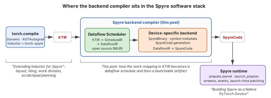
Torch-spyre’s Inductor decides how each kernel’s work is divided across Spyre’s cores and manages tensor residency between on-chip scratchpad and off-chip memory, and the backend compiler turns those decisions into something the hardware can actually run. The contract between them is represented using KTIR (Kernel Tile IR), an MLIR representation built on a data-parallel view of the accelerator, in which every compute tile can see every memory and a single logical tensor can live spread across several cores’ scratchpads. A new open-source Dataflow Scheduler consumes KTIR and turns each tile’s work into a dataflow pipeline: it splits the kernel into programs, starts from a simple load → compute → store pipeline, routes every transfer through the memory hierarchy given in an architecture description, and expands that pipeline into a nested, double-buffered, multi-instance schedule. The output of the scheduler is represented using DataflowIR, an MLIR intermediate representation that Spyre’s device-specific stages use to produce SpyreCode, a symbolic SpyreBinary plus a job plan that the Spyre runtime prepares once and launches many times, filling in tensor addresses and shapes at launch.

This post is the middle chapter of three. Extending Inductor for the IBM Spyre Accelerator described how torch-spyre’s Inductor extensions settle layout, tiling, work division and scratchpad placement, and Building Spyre as a Native PyTorch Device described how the runtime launches a compiled artifact whose symbolic values are only filled in at the last moment. This post covers how the decisions Inductor makes actually become a program the runtime can launch.

Where the backend compiler sits in the Spyre software stack

Three ideas run through the design.

• The frontend decides the parallel decomposition, and the backend makes it run. KTIR is designed to carry the mapping Inductor has already chosen (which core computes what, over which data, out of which memory) so that the backend never has to rediscover it. The backend’s job is dataflow scheduling inside that mapping.
• Scheduling means building a pipeline. Spyre is a dataflow machine with decoupled access and execution, so loads, stores and compute run on separate engines communicating via FIFOs. The scheduler starts from the simplest legal pipeline and refines it one transformation at a time, and every one of those steps is a readable MLIR rewrite.
• The boundary is an IR, not a library call. KTIR, the scheduler’s ScheduleIR and DataflowIR are all ordinary MLIR built on upstream dialects (linalg, scf, arith, memref, tensor), and the scheduler and its dialects are open source under Apache-2.0. Device-specific lowering stages for code generation start at the DataflowIR boundary.

KTIR: the contract between Inductor and the backend

Why a new interface

One of the key requirements for efficient backend scheduling is a contract between torch-spyre’s Inductor and the backend compiler with the capability and flexibility to capture the complete data-parallel view of the accelerator, in which every compute tile can see every memory and a single logical tensor can live spread across several cores’ scratchpads.

KTIR (RFC 0682, implemented in torch-spyre/ktir-mlir-frontend) is a tile-based, block-structured IR built on open-source MLIR. Our goal was to make it expressive enough to capture data-parallel mappings from two quite different sources: Inductor on one side, and hand-written Spyre kernels in languages like Triton or Helion on the other.

A data-parallel abstraction of the accelerator

KTIR is written against a deliberately simple picture of the hardware: a set of cores, each with a compute engine and its own on-chip scratchpad, joined by an on-chip interconnect that also reaches one or more off-chip memories. The property that matters most is that every compute tile has a global view of every memory, which means its own scratchpad, every other core’s scratchpad, and device memory.

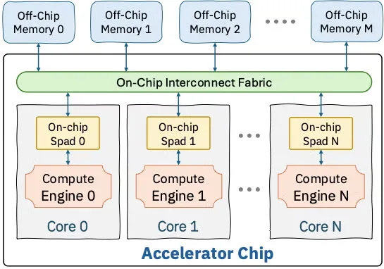
Hardware abstraction of a multi-core accelerator embodied in KTIR (from RFC 0682)

That picture matches Spyre’s shape closely: 32 cores on a ring, each with 2 MB of scratchpad, backed by off-chip device memory. Data moves between device memory and the scratchpads in sticks, fixed 128-byte chunks that hold 64 fp16 values. Intentionally, the picture leaves out details such as FIFOs, load/store units and decoupled execution engines. KTIR describes what each compute tile does and where its data lives, not how that data gets there, because working out how it gets there is exactly the scheduler’s job.

KTIR is also compositional. Arithmetic, reductions and control flow come straight from upstream MLIR dialects (arith, math, linalg, scf, tensor, memref), and a dedicated dialect, ktdp, adds the two things those dialects can’t express: explicit memories and explicit accesses. A second, much smaller dialect, spyreop, covers Spyre’s own intrinsics. The core ktdp operations are:

ktdp op	What it expresses
get_compute_tile_id	Which compute tile this is; 1-D or multi-dimensional, over the grid attribute on the kernel
construct_memory_view	Interpret a region at some (possibly symbolic) address in a named memory space as a strided tensor; no allocation, no data movement
construct_distributed_memory_view	Compose several memory views, each covering part of a global coordinate space, into one logical tensor
construct_access_tile	A structured set of coordinates into a view: an integer set for the domain and an affine map for the traversal order, so tiles can be rectangular, strided, skewed or triangular
construct_indirect_access_tile	The same, with some dimensions indexed through another tensor, e.g. paged KV-cache gathers
load / store	The only data movement: consume an access tile and produce or write a data tile
inter_tile_produce / inter_tile_reduce	Communication between compute tiles, e.g. an all-reduce of partial sums

Here is a complete kernel, an elementwise add over 96×64 fp16 tensors divided among 32 compute tiles of three rows each.

#tile = affine_set<(d0, d1) : (d0 >= 0, -d0 + 2 >= 0, d1 >= 0, -d1 + 63 >= 0)>   // 3x64
#full = affine_set<(d0, d1) : (d0 >= 0, -d0 + 95 >= 0, d1 >= 0, -d1 + 63 >= 0)>
#id   = affine_map<(d0, d1) -> (d0, d1)>

// The tensors' start addresses arrive as arguments: PyTorch's allocator owns them.
func.func @add(%A: index, %B: index, %C: index) attributes {grid = [32]} {
  %c0   = arith.constant 0 : index
  %c3   = arith.constant 3 : index
  %id   = ktdp.get_compute_tile_id : index
  %row0 = arith.muli %id, %c3 : index                 // this tile's 3-row slab

  %A_view = ktdp.construct_memory_view %A, sizes: [96, 64], strides: [64, 1] {
      coordinate_set = #full, memory_space = #ktdp.memory_space<global>
  } : memref<96x64xf16>
  // ... %B_view and %C_view alike

  %A_t = ktdp.construct_access_tile %A_view[%row0, %c0] {
      access_tile_set = #tile, access_tile_order = #id
  } : memref<96x64xf16> -> !ktdp.access_tile<3x64xindex>
  // ... %B_t and %C_t alike

  %a = ktdp.load %A_t : !ktdp.access_tile<3x64xindex> -> tensor<3x64xf16>
  %b = ktdp.load %B_t : !ktdp.access_tile<3x64xindex> -> tensor<3x64xf16>
  %e = tensor.empty() : tensor<3x64xf16>
  %c = linalg.add ins(%a, %b : tensor<3x64xf16>, tensor<3x64xf16>)
                  outs(%e : tensor<3x64xf16>) -> tensor<3x64xf16>
  ktdp.store %c, %C_t : tensor<3x64xf16>, !ktdp.access_tile<3x64xindex>
  return
}

The kernel keeps four concerns apart. Views say how memory should be interpreted, access tiles say which coordinates a given tile touches, loads and stores are the only operations that move data, and linalg does the arithmetic. Notice also that the work division is already settled: grid = [32], together with the arithmetic on %id, is the partitioning, and the backend is expected to honor it rather than second-guess it.

Spyre intrinsics: the spyreop dialect

Upstream arith and math cover most of the arithmetic a kernel needs, but Spyre’s compute units also offer operations that no generic dialect has a name for. A kernel that wants one of those should be able to ask for it directly, instead of hoping the backend recognizes some particular pattern of arith ops. For that, KTIR comes with a second, much smaller dialect, spyreop, which exposes Spyre intrinsics as ordinary MLIR operations. It covers elementwise and activation functions (exp, gelu, sigmoid, silu, softplus, sqrt, rsqrt, reciprocal, realdiv), the building blocks of normalization (a combined mean and mean of squares, and the normalizing and scaling halves of LayerNorm, some with fused variants), integer and address arithmetic (including idx32toaddr, which computes base + stride × index for gathers), and compare and select. The dialect also defines df16, IBM’s 16-bit DLFloat format, which splits its bits 1-6-9 between sign, exponent and mantissa rather than IEEE half precision’s 1-5-10, along with “fused” types that carry a pair of floats as a single value.

Intrinsics appear wherever any other scalar computation would, which is inside the body of a linalg.generic:

%y = linalg.generic {indexing_maps = [#in, #out],
                     iterator_types = ["parallel", "parallel", "parallel", "parallel"]}
       ins(%x : tensor<6x64x64xf16>) outs(%init : tensor<1x6x64x64xf16>) {
  ^bb0(%a: f16, %out: f16):
    %g = spyreop.gelu %a : f16
    linalg.yield %g : f16
} -> tensor<1x6x64x64xf16>

Because they are just operations in a linalg body, intrinsics fuse with the surrounding elementwise work like anything else, and the scheduler carries them through as compute until it is ready to lower them. How each intrinsic expands into the hardware’s own instruction sequence is not written in the scheduler at all: it lives in the architecture description, as one of the device patterns described later in this post.

How KTIR captures Inductor’s work mapping

The Inductor post walked through a series of decisions torch-spyre makes before any code is generated. Each of them has a direct counterpart in KTIR:

Decision in torch-spyre’s Inductor passes	How it appears in KTIR
Work division: the per-op core split, e.g. a matmul’s 16 × 2 grid	The kernel’s grid attribute, plus affine arithmetic on ktdp.get_compute_tile_id that picks each tile’s slice
Stick-granularity layout: which dimension is the stick, and the tiled order of the others	Strides of construct_memory_view, and the access_tile_order of each access tile
Coarse tiling and working-set reduction	scf.for loops around loads, compute and stores, which run the chain tile by tile
Scratchpad residency chosen by the scratchpad allocator	A memory view in #ktdp.memory_space<ct_local, ct_id = k> at the offset the allocator assigned
A tensor split across cores so each slice fits in scratchpad	construct_distributed_memory_view over per-core ct_local views
Core-to-core relayout (lx_relayout)	An access tile over one distributed view, stored into a view with a different distribution
Reduction split across cores (partial sums of one output tile)	inter_tile_produce / inter_tile_reduce
Paged tensors and gathers	construct_indirect_access_tile
Device-specific activations and normalization steps	spyreop intrinsics inside linalg.generic bodies
Tensor addresses owned by PyTorch’s allocator	Kernel arguments. They stay symbolic all the way to SpyreCode and are substituted by the runtime at launch
Tensor shapes known only at runtime, within a bound	!ktdp.runtime_arg<index, granularity = G, upperbound = U>, kept symbolic and substituted at launch in the same way

The last two rows are where this post meets the runtime post. Because KTIR allows a start address or a size to be a value rather than a constant, every layer beneath it can keep that value symbolic until the runtime is in a position to supply it.

Tensors pinned in scratchpad, distributed across cores

What most sets KTIR apart from GPU-oriented tile IRs is the way it treats on-chip memory. A tile language like Triton describes each program instance loading blocks of a tensor from global memory, computing on them, and storing the results back. How those blocks are staged through shared memory, registers and caches is left to the compiler and the hardware, and a program instance’s on-chip storage is private to it and lives only as long as it runs. In that model there is typically no way, and little need, to say that a tensor should still be sitting in a particular core’s on-chip memory when the next operation reads it, or that one program instance should read data held on-chip by another. That works well on hardware where caches and a dynamic scheduler smooth over data movement. It doesn’t fit Spyre. There is no hardware-managed cache to fall back on, and keeping a tensor on-chip from one operation to the next is one of the biggest performance levers available. On Spyre, the scratchpad isn’t a cache that a kernel happens to hit; it’s memory the compiler chooses to use, with Inductor’s scratchpad allocator deciding which buffers stay resident, at what address and on which core. KTIR therefore makes on-chip placement a first-class part of the IR rather than an implementation detail: it simply writes that decision down.

Each memory space names a physical memory: #ktdp.memory_space<global> is device memory, and #ktdp.memory_space<ct_local, ct_id = k> is the scratchpad belonging to compute tile k. A view’s coordinate_set records which part of a larger logical tensor it holds, so if you combine per-core views with construct_distributed_memory_view, you get a single tensor, indexed by global coordinates, whose storage is spread across several scratchpads.

// X[128, 1024] f16, left in scratchpad by an earlier op of the kernel:
// 32 rows on each of four cores, at the offset the scratchpad allocator chose.
#rows0 = affine_set<(d0, d1) : (d0 >= 0,      -d0 + 31 >= 0,  d1 >= 0, -d1 + 1023 >= 0)>
#rows1 = affine_set<(d0, d1) : (d0 - 32 >= 0, -d0 + 63 >= 0,  d1 >= 0, -d1 + 1023 >= 0)>
// ... #rows2, #rows3

%X0 = ktdp.construct_memory_view %lx_off, sizes: [32, 1024], strides: [1024, 1] {
        coordinate_set = #rows0, memory_space = #ktdp.memory_space<ct_local, ct_id = 0>
      } : memref<32x1024xf16>
%X1 = ktdp.construct_memory_view %lx_off, sizes: [32, 1024], strides: [1024, 1] {
        coordinate_set = #rows1, memory_space = #ktdp.memory_space<ct_local, ct_id = 1>
      } : memref<32x1024xf16>
// ... %X2, %X3
%X = ktdp.construct_distributed_memory_view (%X0, %X1, %X2, %X3
        : memref<32x1024xf16>, memref<32x1024xf16>, memref<32x1024xf16>, memref<32x1024xf16>)
        : memref<128x1024xf16>

// Compute tile 1 reads rows 48-79: half from its own scratchpad, half from core 2's.
#rows32 = affine_set<(d0, d1) : (d0 >= 0, -d0 + 31 >= 0, d1 >= 0, -d1 + 1023 >= 0)>
%id  = ktdp.get_compute_tile_id : index
%row = affine.apply affine_map<(d0) -> (d0 * 32 + 16)>(%id)
%t = ktdp.construct_access_tile %X[%row, %c0] {
       access_tile_set = #rows32, access_tile_order = #id
     } : memref<128x1024xf16> -> !ktdp.access_tile<32x1024xindex>
%x = ktdp.load %t : !ktdp.access_tile<32x1024xindex> -> tensor<32x1024xf16>

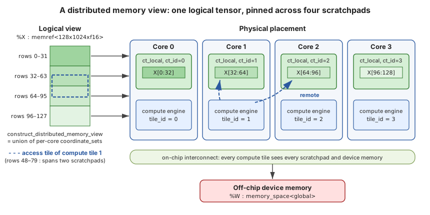A distributed memory view: one logical tensor, pinned across four scratchpads

This one construct does quite a lot of work. First, it lets intermediate tensors stay on-chip from one operation to the next: a producer can store into a distributed ct_local view and a consumer can load from it without either of them ever mentioning device memory, which is precisely the kind of fusion without a round trip that the softmax example in the Inductor post was built around. Second, it turns a core-division mismatch into ordinary IR. When a producer and a consumer divide a tensor differently, the consumer’s access tiles just cross scratchpad boundaries, and since every compute tile can see every scratchpad, that is still nothing more than a load; the on-chip relayout that torch-spyre’s co-optimizing allocator weighs against a spill needs no special-purpose op. Third, it keeps placement binding. The runtime post argued that “placement must be explicit and binding because compiled code may depend on it,” and KTIR is where that dependency is recorded, since the memory space and coordinate set on a view are the placement contract.

The backend compiler at a glance

The backend compiler is a single MLIR pipeline in two halves. The open-source Dataflow Scheduler lowers KTIR through ScheduleIR to DataflowIR, and three device-specific stages (symbolic SpyreBinary generation, metadata generation for runtime symbol substitution, and SpyreCode generation) then turn DataflowIR into SpyreCode. DataflowIR is the only point where the two halves meet.

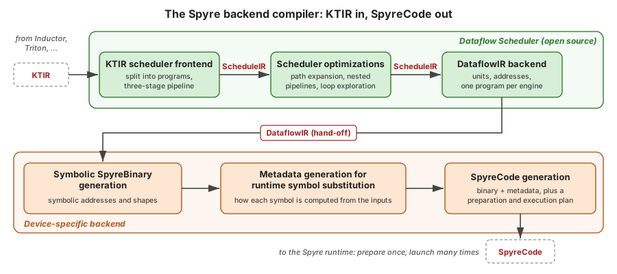The Spyre backend compiler: KTIR in, SpyreCode out

The rest of the post follows the figure from left to right, spending most of its time on the scheduler and then covering the three stages below it more briefly.

The Dataflow Scheduler: KTIR → ScheduleIR → DataflowIR

A dataflow accelerator is a distributed collection of compute engines and scratchpad memories connected by wide datapaths with FIFOs. It follows a decoupled access-execute design, in which moving data (DMA, scratchpad loads and stores) and computing on it happen on separate engines that run at the same time. On a machine like that, scheduling means building a dataflow pipeline across space and time, deciding which engine performs each step and how the steps overlap with one another.

The Dataflow Scheduler does this as an MLIR pass pipeline, and a handful of principles shape how it’s built. It is driven by an architecture description rather than hard-coded for one chip, which we look at more closely below. Every schedule is expressed in a single execution model built from just three constructs: nested scf.for loops, ktdf.pipeline (stages that overlap across iterations) and ktdf.parallel (identical instances that split an iteration space between them), and every analysis and transformation reasons in those terms. Wherever it can, the scheduler leans on upstream MLIR, lowering compute to linalg.generic and fusing it with upstream passes, and using scf for loops and memref for buffers. And throughout, it follows one strategy: start with the most naive correct pipeline, then let each later pass either make it legal on the hardware or make it bigger, in small steps that can be tested on their own.

The passes fall into three groups, each with a fixed IR contract at its boundaries, so passes can be added or reordered within a group without disturbing the others.

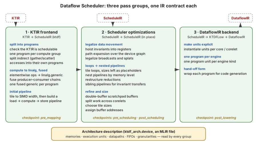Dataflow Scheduler: three pass groups, one IR contract each

At four named checkpoints (pre_mapping, pre_scheduling, post_scheduling and post_lowering) the scheduler applies rewrite patterns written in PDL. Those patterns live in the architecture description rather than in the scheduler, which means a device can supply its own lowerings without forking the scheduler. This is where each spyreop intrinsic, such as spyreop.exp or spyreop.gelu, is replaced by the hardware’s instruction template, and where an inner-dimension reduction becomes a SIMD reduction.

The scheduler’s intermediate form, ScheduleIR, is the ktdf dialect used alongside linalg, scf and memref. Its vocabulary is small enough to list in full:

ktdf construct	Meaning
ktdf.pipeline [modulo(size: N)]	A chain of stages that overlap across iterations; modulo rotates through N copies of its resources (N-buffering)
ktdf.stage depends_in(...) depends_out(...)	One step of a pipeline, eventually bound to one kind of execution unit (applicable_units)
ktdf.private	Resources private to one pipeline: FIFO slots, scratchpad buffers, tokens
!ktdf.token	A pure ordering value between stages, with no runtime cost of its own
!ktdf.fifo.slot<SRC -> DST, 64xf16>	A slot in a hardware FIFO between two units
ktdf.data_transfer / ktdf.ind_data_transfer	Explicit movement between memories and FIFOs, direct or through an indirect-address buffer
ktdf.read_from_fifo / ktdf.write_to_fifo	How a compute stage consumes and produces FIFO data
ktdf.parallel ... distribute(num_instances = N)	Split an iteration space into contiguous blocks over N identical hardware instances
ktdf.tiling.reserve_size / derive_size / linearize_index	Placeholders for tile sizes chosen later, the current tile’s extent, and the original index

The architecture description

Everything the scheduler knows about the hardware comes from a single MLIR file written in the ktdf_arch dialect. That file describes the device as a graph. Its nodes are memories, with their kinds and sizes, and execution units, with the features the scheduler cares about: SIMD lane counts per element type, the word sizes and access granularities of load and store units, the depth of each FIFO. Its edges are datapaths, each with a transfer granularity. Groups scope resources the way the hardware does, for example a core that owns a scratchpad along with the load/store and compute units that use it. Here is a trimmed and simplified version of the sample device used in the scheduler’s tests:

#L1  = { kind = "L1", size = 1048576 }                           // 1 MB scratchpad
#SFU = { kind = "SFU", ktdf_arch.features = {
           ktdf_arch.feature.compute,
           ktdf_arch.feature.simd = { lanes = #ktdf_arch.map<f16 = 64, f32 = 32, i32 = 32> } } }
#L1LU_CORE_FIFO = { ktdf_arch.features = { ktdf_arch.feature.queue = { depth = 16, ordered } } }

ktdf_arch.device @sample_device {
  %ddr = memory #DDR
  group { kind = "core" } share(%ddr) {
    %l1 = memory #L1
    %mnilu = group { kind = "MNILU_Block" } share() { ... } -> exec_unit   // DMA load unit
    %mnisu = group { kind = "MNISU_Block" } share() { ... } -> exec_unit   // DMA store unit
    datapath #DDR_MNILU %ddr to %mnilu : memory, exec_unit
    datapath #MNILU_L1 %mnilu to %l1 : exec_unit, memory
    %sfu  = group { kind = "SFU_Block" } share() { ... } -> exec_unit   // compute unit
    %l1lu = exec_unit #L1LU                                              // scratchpad load unit
    %l1su = exec_unit #L1SU                                              // scratchpad store unit
    datapath #L1LU_CORE_FIFO %l1 to %l1lu : memory, exec_unit
    datapath %l1lu to %sfu : exec_unit, exec_unit
    ...
  }
  patterns ["pre_scheduling"] { ... }                   // device-specific rewrites, in PDL
  patterns ["post_scheduling"] { ... }
}

A kernel refers to its target with a one-line declaration that imports this file and maps KTIR’s memory spaces onto the device’s memories, for example global onto DDR and ct_local onto L1. From then on, nearly every decision in the pipeline reads something from the description. The SIMD lane count sets the width of the first pipeline. The datapaths form the routing graph that path expansion searches, so the hops a transfer takes are whatever the graph allows. Access granularities, transfer granularities and FIFO depths constrain how each transfer can be shaped. Memory sizes bound what address assignment can place, and therefore which tile sizes fit. And the patterns blocks supply the device’s own lowerings, such as how each spyreop intrinsic expands into the hardware’s instructions, at the scheduler’s checkpoints.

Because all of that lives in the description rather than in the passes, retargeting the scheduler means writing a new description, not changing the scheduler. Spyre has its own description, the scheduler’s tests run against the sample device above, and the same passes run unchanged on both.

Step 1: Break the kernel into programs

A KTIR kernel is a sequence of operations, whereas a Spyre program is a single pipeline configuration loaded onto the device, so the scheduler’s first real decision is where to cut the kernel into separately scheduled programs.

The scheduler makes that cut by working backwards from each ktdp.store, through the compute that feeds it, to the ktdp.loads it ultimately depends on. Everything connected that way forms one compute group, a single load → compute → store chain through memory, and a group ends either at a load that belongs to a different group or at any operation with a region, such as a loop or a conditional. Each group then becomes its own nested MLIR module, module @local_schedule_N, while the original kernel turns into an orchestrator that keeps the control flow and address arithmetic and calls the programs in order. The number of programs is therefore exactly the number of compute groups.

// KTIR: loads, compute and stores interleaved with a loop nest
func.func @kernel() {
  scf.for %i = %c1 to %c5 step %c1 {
    ... ktdp.load A ... linalg.add ... ktdp.store B ...
    scf.for %j = %c1 to %c3 step %c1 {
      ... ktdp.load B ... linalg.mul ... ktdp.store C ...
    }
    ... ktdp.load C ... linalg.sub ... ktdp.store D ...
  }
}

// ScheduleIR: an orchestrator that calls one program per compute group
module {
  func.func @kernel() {
    scf.for %i = %c1 to %c5 step %c1 {
      func.call @local_schedule_1() : () -> ()
      scf.for %j = %c1 to %c3 step %c1 {
        func.call @local_schedule_0() : () -> ()
      }
      func.call @local_schedule_2() : () -> ()
    }
    return
  }
  func.func private @local_schedule_0()
  ...
}
module @local_schedule_0 { func.func @local_schedule_0() { /* views, tile id, load, mul, store */ } }
module @local_schedule_1 { ... }
module @local_schedule_2 { ... }

One consequence of this split is worth spelling out, because it separates two very different kinds of loop. Loops that appear in the KTIR, which usually come from Inductor’s coarse tiling, stay in the orchestrator and become a sequence of program launches over tiles. Loops inside a program, on the other hand, belong to the scheduler: it creates them by tiling the fused compute down to the hardware’s vector width, and it is free to restructure them however it likes.

Each program also takes its own copy of whatever it needs from the kernel, including the memory views, the constants, ktdp.get_compute_tile_id and the grid attribute, so Inductor’s work division reaches every program intact. Kernels with indirect accesses get split one step further: the first program converts indices into addresses (with spyreop.idx32toaddr) in an indirect-address buffer, and the second uses that buffer to perform the gather or scatter. Finally, within each program, elementwise ops are converted to linalg, generalized to linalg.generic, and fused along producer–consumer chains, leaving every program with exactly one fused linalg.generic, which is the unit the rest of the scheduler works on.

Step 2: The simplest pipeline that could work

Next, the scheduler gives each program its first dataflow pipeline. It tiles the fused generic to the SIMD width of the default compute unit, which it reads from the architecture description (64 lanes of fp16 on the sample device), tags each resulting loop as either a parallel_loop or a reduction_loop, and then builds a three-stage ktdf.pipeline in the innermost loop that loads from memory into a FIFO, computes, and stores from a FIFO back to memory.

scf.for %i ... { scf.for %j ... {
  ktdf.pipeline {
    %p:6 = ktdf.private -> (!ktdf.fifo.slot<"DDR" -> "SFU", 64xf16>, !ktdf.fifo.slot<"DDR" -> "SFU", 64xf16>,
                            !ktdf.fifo.slot<"SFU" -> "DDR", 64xf16>, !ktdf.token, !ktdf.token, !ktdf.token) {...}
    ktdf.stage depends_in(none) depends_out(%p#3) {
      ktdf.data_transfer from %A[%i, %j] size [1, 64] to %p#0 size [1, 64] : ...
      ktdf.data_transfer from %B[%i, %j] size [1, 64] to %p#1 size [1, 64] : ...
    }
    ktdf.stage depends_in(%p#3) depends_out(%p#4) {
      %a = ktdf.read_from_fifo %p#0 : <"DDR" -> "SFU", 64xf16> -> tensor<1x64xf16>
      %b = ktdf.read_from_fifo %p#1 : <"DDR" -> "SFU", 64xf16> -> tensor<1x64xf16>
      %r = linalg.generic {...} ins(%a, %b : ...) outs(%e : tensor<1x64xf16>) {...}
      ktdf.write_to_fifo %r, %p#2 : tensor<1x64xf16>, <"SFU" -> "DDR", 64xf16>
    } {applicable_units = ["SFU"]}
    ktdf.stage depends_in(%p#4) depends_out(%p#5) {
      ktdf.data_transfer from %p#2 size [1, 64] to %C[%i, %j] size [1, 64] : ...
    }
  }
} {loop_type = #ktdf.loop_type<parallel_loop>} } {loop_type = #ktdf.loop_type<parallel_loop>}

(The snippets in this section are taken from the scheduler’s lit tests, which use a sample architecture whose memories are called DDR and L1 and whose compute unit is called SFU. On Spyre, the same roles are played by device memory, each core’s scratchpad and its compute pipelines.)

This pipeline is functionally complete, but it isn’t legal yet, since nothing in the hardware connects device memory straight to the compute engine through a FIFO. Fixing that is the first job of the next pass group.

Step 3: Path expansion routes data through the memory hierarchy

Path expansion legalizes data movement using the architecture description. It builds a routing graph from the device, with memories, execution units and load/store units as nodes and datapaths as edges, and then, for each pipeline, takes the endpoints implied by the three-stage version (device memory → compute → device memory, for instance), runs a shortest-path search between each consecutive pair, and stitches the hops together. Wherever the real path turns out to be longer than the endpoints suggested, the pass rewrites the pipeline, inserting a transfer stage for each intermediate hop, allocating staging buffers in scratchpad, retyping the FIFOs so that each one connects two units that are actually adjacent, and tagging every stage with the kind of unit that will execute it.

In the example, three stages become five: a DMA load unit brings a tile into scratchpad, a scratchpad load unit feeds it into the FIFO, the compute engine consumes and produces, a scratchpad store unit drains the result FIFO, and a DMA store unit writes the result back.

ktdf.pipeline {
  %p:10 = ktdf.private -> (memref<1x64xf16, "L1">, memref<1x64xf16, "L1">,
                           !ktdf.fifo.slot<"L1LU" -> "SFU", 64xf16>, ..., !ktdf.fifo.slot<"SFU" -> "L1SU", 64xf16>,
                           memref<1x64xf16, "L1">, !ktdf.token, ...) {...}
  ktdf.stage ... { ktdf.data_transfer from %A[%i, %j] ... to %p#0[0, 0] ... }  {applicable_units = ["MNILU"]} // DDR -> L1
  ktdf.stage ... { ktdf.data_transfer from %p#0[0, 0] ... to %p#2 ... }         {applicable_units = ["L1LU"]}  // L1 -> FIFO
  ktdf.stage ... { ... read_from_fifo ... linalg.generic ... write_to_fifo ... } {applicable_units = ["SFU"]}   // compute
  ktdf.stage ... { ktdf.data_transfer from %p#4 ... to %p#5[0, 0] ... }         {applicable_units = ["L1SU"]}  // FIFO -> L1
  ktdf.stage ... { ktdf.data_transfer from %p#5[0, 0] ... to %C[%i, %j] ... }  {applicable_units = ["MNISU"]} // L1 -> DDR
}

This is also where the placement information in KTIR starts to pay off. If an operand is already a ct_local view, meaning Inductor pinned it in scratchpad, then its path to the compute engine starts at the scratchpad, and path expansion adds no DMA stages for it at all. The pipeline runs straight from scratchpad to FIFO to compute, and the tensor never takes a round trip through device memory. In other words, residency decided in Inductor becomes pipeline structure in the scheduler without any extra machinery in between.

A few follow-up legalizations round this out: indirect-address-buffer fills are staged through a memory that the filling unit can actually read, and scalar operands are widened to full vector width and transferred as hardware splats.

Step 4: Nested pipelines, one level of the memory hierarchy at a time

After path expansion, every stage still runs once per 64-element vector. That’s legal, but wasteful: DMA engines move data most efficiently in bulk, and the whole point of the scratchpad is to have data waiting before the compute needs it. The scheduler therefore reshapes the program’s loop nest into a hierarchy of pipelines, each running at the granularity that suits its own level of the memory hierarchy.

It starts by tiling the parallel loops into tile loops and point loops, but leaves each tile size as a placeholder in the IR (ktdf.tiling.reserve_size), with its constraints attached, so the size itself can be chosen later. It then works out which stages have to move in lockstep, because they talk through a FIFO or through registers, and which don’t, like a DMA stage that only touches device memory and scratchpad. The loops over a tile are sunk into those groups. A DMA stage becomes a single bulk transfer of the whole tile into scratchpad, while the scratchpad-load → compute → scratchpad-store chain becomes one stage that contains its own nested ktdf.pipeline. What you end up with is an outer pipeline that works a tile at a time, wrapped around an inner pipeline that works a vector at a time.

Not every new pipeline is nested. Transfers that don’t change from one iteration of a loop to the next, such as an operand broadcast along that loop’s dimension or a constant buffer, are hoisted into a sibling pipeline that runs once before the loop, instead of refetching the same data on every iteration. Reductions are restructured in the same spirit: large ones are chunked to fit in scratchpad, the outer part becomes an explicit loop with a carried accumulator, and the innermost, stick-width part is left for a device pattern to map onto the hardware’s own reduction support.

scf.for %m0 ... { scf.for %n0 ... {
  ktdf.pipeline {                                            // outer: tile granularity
    %p0:5 = ktdf.private -> (memref<2x1x64xf16, "L1">, ..., !ktdf.token, !ktdf.token) {...}
    ktdf.stage depends_in(none) depends_out(%p0#3) {         // bulk DDR -> L1 for the tile
      scf.for %m1 ... { scf.for %n1 ... { ktdf.data_transfer from %A[..] ... to %p0#0[..] ... } }
    }
    ktdf.stage depends_in(%p0#3) depends_out(%p0#4) {        // compute stage holds a pipeline
      scf.for %m1 ... { scf.for %n1 ... {
        ktdf.pipeline {                                      // inner: vector granularity
          ktdf.stage ... { ktdf.data_transfer from %p0#0[..] ... to %fifo_in ... }   // L1 -> FIFO
          ktdf.stage ... { ... linalg.add ... }                                      // compute
          ktdf.stage ... { ktdf.data_transfer from %fifo_out ... to %p0#2[..] ... }  // FIFO -> L1
        }
      } }
    }
    ktdf.stage depends_in(%p0#4) depends_out(none) {         // bulk L1 -> DDR
      scf.for %m1 ... { scf.for %n1 ... { ktdf.data_transfer from %p0#2[..] ... to %C[..] ... } }
    }
  }
} }

Step 5: Exploring the loop space

Once the pipeline’s shape is settled, the remaining question is how much of it runs at once. Scratchpad buffers that one stage writes and another reads inside a loop are double-buffered, so the pipeline rotates between two copies (modulo(size: 2)) and the DMA stage can fill tile N+1 while compute is still draining tile N. That is exactly the load/compute overlap the decoupled design exists to provide. Work is then split across the sub-core instances (corelets) inside each core, with a parallel loop around a corelet-local pipeline becoming a ktdf.parallel ... distribute(num_instances = N) and N taken from the architecture description. This gives a second level of parallelism, inside each of the cores that Inductor’s grid has already assigned. Only after that are the tile-size placeholders filled in, so that the sizes chosen already account for the parallel instances.

Taken together, this is a genuine loop space. Loop structure, pipeline granularity, buffering depth, instance split and tile size are all separate, explicit decisions in the IR, each bounded by what the architecture description allows. We want to be clear about where this stands today, though: in the V1 scheduler, these choices are made by local heuristics rather than by search or a cost model. Keeping every choice explicit in the IR, as placeholders, modulo factors and distribute counts, was deliberate, so that a cost model or an autotuner can be added later without touching the structure of the pipeline.

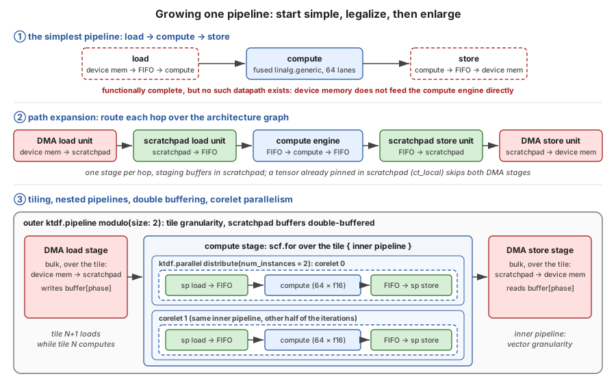Growing one pipeline: start simple, legalize, then enlarge

Step 6: Addresses, units and DataflowIR

The last stretch turns the logical schedule into a concrete one. Every buffer gets an address in its memory, checked against the capacities in the architecture description. Scratchpad is allocated per program, while device-memory allocations persist across programs, since that’s how one program hands its results to the next. The abstract unit kinds are then instantiated for each core (and for each corelet, where the work is parallel), token dependencies become explicit signals, and each program is split into one dataflow.program_unit per kind of engine, each keeping only the part of the work that runs on it. Along the way, transfers become address-generation and send/receive operations, and the compute tile id becomes a per-core lookup. Each program ends up with two levels: an outer function with the program’s real signature, which declares its symbols, and an inner, argument-free function that holds the DataflowIR.

Symbolic values, whether tensor addresses or tensor shapes, make it through all of this intact. Taking an address as the example, a start address computed from a kernel argument becomes a symbol.create_symbol with an ID, and the expression that produces it (the argument plus this grid element’s share of the tensor, converted to the unit’s address granularity) is recorded one level up with symbol.create_id. When different grid elements start at different offsets, each one gets its own symbol, selected through a per-unit map.

// One level up: what each symbol is, as arithmetic over the kernel argument
func.func @local_schedule_0(%base: index) {
  symbol.create_id %base {symbol_id = -1}
  %w0 = arith.divsi %base, %c64 : index                   // grid element 0, in 64-byte words
  symbol.create_id %w0 {symbol_id = -2}
  %b1 = arith.addi %base, %c49152 : index                 // grid element 1: base + its slab
  %w1 = arith.divsi %b1, %c64 : index
  symbol.create_id %w1 {symbol_id = -3}
  call @local_schedule_0_body() : () -> ()
}
// The DataflowIR itself takes no arguments; it only names symbols.
%s0 = symbol.create_symbol {SymbolId = -2 : i64} : index
%s1 = symbol.create_symbol {SymbolId = -3 : i64} : index
%m  = uniform.def_immutable_mapping([%core0 -> %s0], [%core1 -> %s1]) : index
%a  = uniform.query_map(map: %m, key: %unit) : index
dataflow.get_logical_memory_view %ddr, %a ...

The resulting table of symbols, each written as an expression over the kernel’s inputs, is what the runtime eventually evaluates at launch.

DataflowIR is the hand-off point, consisting of per-engine program units built from the dataflow, vectorchain, agen, uniform, symbol and scf dialects. This is where the open-source scheduler stops, and its only obligation to what comes next is to emit valid DataflowIR in those dialects with stable program-unit tags.

From DataflowIR to SpyreCode

The remaining stages are device-specific, so we describe them only as far as is needed to connect this post with the runtime post.

Symbolic SpyreBinary generation lowers each program’s DataflowIR into a SpyreBinary: the binary that configures and starts the program’s units on the device. Any value that depends on the caller’s tensors, whether a tensor address or a tensor shape, stays in the binary as a symbol. Metadata generation for runtime symbol substitution then records how each of those symbols is computed from the kernel’s inputs. Finally, SpyreCode generation packages the SpyreBinary and its metadata together with a job plan in two parts.

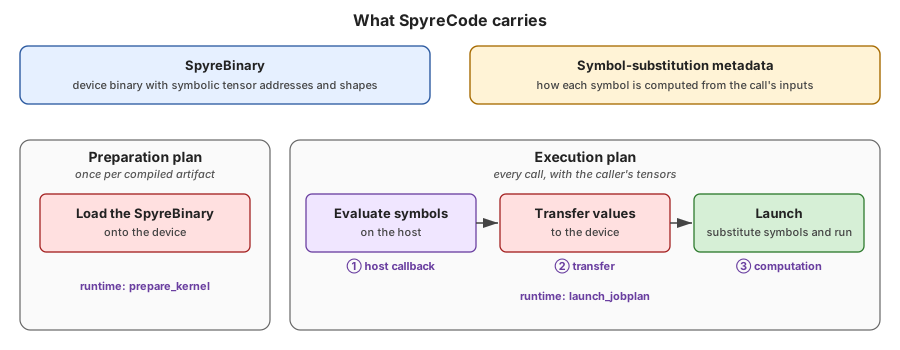What SpyreCode carries: a symbolic SpyreBinary, its symbol-substitution metadata, and a two-phase job plan

Those two parts line up with the split the runtime post draws between preparation and launch. The preparation plan loads the SpyreBinary onto the device and doesn’t depend on the call’s arguments, so the runtime’s prepare_kernel runs it once. The execution plan evaluates the symbols over the actual tensor addresses and shapes on the host, transfers the resolved values to the device, and launches the computation, which are the runtime post’s three launch-time steps in order. launch_jobplan walks it on every call, and a kernel whose addresses and shapes are all known at compile time needs only the launch.

Try it

The Dataflow Scheduler builds against upstream LLVM/MLIR. The README gives the exact LLVM revision and how to build it. With an MLIR build in place, the scheduler takes a couple of commands:

git clone --recursive https://github.com/torch-spyre/dataflow-scheduler.git
cd dataflow-scheduler
cmake -S . -B build -G Ninja -DMLIR_DIR=$MLIR_INSTALL_PREFIX/lib/cmake/mlir
cmake --build build

A good hello world is the simple elementwise add in the repository’s tests, test/dataflow-scheduler-opt/ktir-to-dfir-sanity-check.mlir. It is a small, self-contained KTIR kernel, much like the add from earlier in this post, split across two compute tiles and targeting the sample device described above. Running the whole pipeline on it prints the DataflowIR it produces:

./build/bin/dataflow-scheduler-opt -ktir-to-dfir \
    test/dataflow-scheduler-opt/ktir-to-dfir-sanity-check.mlir

Adding --mlir-print-ir-after-all shows the IR after every pass, which is the easiest way to watch the program split, the three-stage pipeline appear, path expansion insert its hops, and the pipelines nest. For your own kernels and devices, the dataflow-scheduler driver takes the architecture description directly, as dataflow-scheduler -kEmitDFIR --device=<path-to-device.mlir> <kernel.mlir>, and writes the resulting DataflowIR to files.

Conclusion

Taken together, the three posts trace a single path from torch.compile down to Spyre silicon. Inductor decides the layout, the tiling, the division of work across cores, and which tensors stay pinned in scratchpad. KTIR records those decisions in MLIR, as compute tiles, explicit memories, distributed views, access tiles and Spyre intrinsics, without committing to any dataflow detail. The Dataflow Scheduler then makes them run, cutting the kernel into programs, building a pipeline, routing each transfer through the memory hierarchy, and nesting, buffering and parallelizing that pipeline, all guided by an architecture description rather than hard-coded knowledge of one chip. The device-specific stages turn the result into SpyreCode, a symbolic SpyreBinary plus a two-phase job plan whose tensor addresses and shapes can stay symbolic until launch, and the runtime prepares it once and launches it on every call through ordinary PyTorch streams.

Every boundary along that path is an IR, and each IR states the facts the next stage needs: placement in KTIR, pipelines in ScheduleIR, per-engine programs in DataflowIR, and the preparation/execution split in SpyreCode. Making those facts explicit is ultimately what allows a dataflow accelerator to sit behind PyTorch’s ordinary interfaces.

Version 1 of the Dataflow Scheduler is ready. It handles elementwise operations with broadcast and reduction dimensions across multi-core KTIR programs, and it has been validated end to end, from KTIR through scheduling and code generation, on representative transformer operations. One of the clearest benefits so far has been how much less developer time it takes to bring up an op: the first op we enabled came up about 4x faster than on the previous stack, and subsequent ops about 8x faster. The same approach has also given us working paths from both the Inductor and Triton frontends. Next, we are completing matrix multiplication support in the Dataflow Scheduler and adding cost-model-driven performance optimizations, with the goal of running LLMs end to end.

KTIR and the Dataflow Scheduler are open source, and the Try it section above is the quickest way to see the pipeline in action. If you’re building a compiler for a dataflow or scratchpad-based accelerator, we’d love to hear from you, since the architecture-description approach is meant to make the scheduler useful well beyond Spyre.

The post From KTIR to SpyreCode: An MLIR Dataflow Backend for IBM Spyre appeared first on PyTorch.